상대적인 가격의 수준을 가지고 트레이딩을 해보자는 아이디어로 몇 가지 조건들을 넣고 최적화를 해봤다. 처음에 의도했던 것은 이런 게 아니었는데 Sharp가 높은 방향으로 흐르다 보니 역추세전략이 만들어졌다. 대략적으로 테스트해 보면 QQQ, SPY는 물론 NQ, ES 같은 선물차트에도 잘 통한다. 아래 코드는 NQ에 적용하기 위해서 시그널 발생 이후 익일 시가에 진입하는 버전으로 구성한 것.
거래방법을 간략히 설명하면 rpsi지표를 만들고 지표가 일정 밑으로 떨어지고 Volatility가 threshold 이내에 존재할 경우에 비중조절을 통해서 진입, 비중조절은 rpsi값을 통해 계산, rpsi가 회복되면 자연스럽게 청산함.


평균 보유기간이 약 2일 수준 가량 된다. 분봉 단위로 쪼개서 당일 청산을 하거나 손절을 조건에 추가하게 되면 약간의 개선점이 있는데 문제는 기존에 보유하고 있던 전략과 상관관계가 높은데 반해서 퍼포먼스는 조금 떨어진다. 아마 슬리피지를 고려하면 조금 더 하락할 수도 있다. 몇 가지 파라미터들을 조절해 봤는데 CAGR은 최대가 6% 수준이고 MDD는 -10% 정도 되는 듯.
기존 전략을 대체하기가 어려워 활용도를 고민중인데 아마도 전일 미국장의 흐름에 따라 아침에 단기적으로 국내 시장에서 ETF를 얼마나 사야 하는지와 같은 보조적인 비중 지표로 활용될 수 있지 않을까 싶다.
import numpy as np
import pandas as pd
import matplotlib.pyplot as plt
from dataclasses import dataclass
# =============== Helper Functions ===============
def compute_rpsi_for_window(df: pd.DataFrame, window: int,
close_col="close", high_col="high", low_col="low") -> pd.Series:
"""RPSI with breakout extension (can go above 1 / below 0)."""
close = df[close_col].astype(float)
high = df[high_col].rolling(window, min_periods=1).max()
low = df[low_col].rolling(window, min_periods=1).min()
eps = 1e-12
rpsi = (close - low) / (high - low + eps)
rpsi = np.where(close > high, 1 + (close - high) / (high + eps), rpsi)
rpsi = np.where(close < low, (close - low) / (low + eps), rpsi)
return pd.Series(rpsi, index=df.index, name=f"rpsi_{window}")
def annualized_return(returns: pd.Series, periods_per_year=252) -> float:
r = returns.dropna()
if len(r) == 0:
return np.nan
yrs = len(r) / periods_per_year
return r.sum() / yrs
def sharpe_ratio(returns: pd.Series, rf=0.0, periods_per_year=252) -> float:
r = returns.dropna()
sd = r.std()
if sd == 0 or np.isnan(sd):
return np.nan
return (r.mean() - rf/periods_per_year) / sd * np.sqrt(periods_per_year)
def max_drawdown(equity: pd.Series) -> float:
peak = equity.cummax()
dd = equity - peak
return float(dd.min())
def trades_count(weight: pd.Series) -> int:
"""Entry = weight goes from 0 → >0."""
w = weight.fillna(0)
return int(((w > 0) & (w.shift(1) == 0)).sum())
def avg_holding_days(weight: pd.Series) -> float:
"""Average length of contiguous >0 weight segments."""
w = (weight.fillna(0) > 0).astype(int)
blocks = (w != w.shift()).cumsum()
lengths = w.groupby(blocks).sum()
lengths = lengths[lengths > 0]
return float(lengths.mean()) if len(lengths) else np.nan
# =============== Parameters Dataclass ===============
@dataclass
class Params:
rpsi_window: int = 2
threshold: float = 0.4
sma_period: int = 8
vol_window: int = 20
z_limit: float = 2.0
lag_days: int = 1 # T+1 execution
csv_path: str = "test.csv"
show_plots: bool = True
weight_step: float = 0.2
fixed_ratio: float = 0.0
# =============== Core Strategy ===============
def run_strategy(price_df: pd.DataFrame, params: Params) -> dict:
df = price_df.copy().sort_values("date").reset_index(drop=True)
df.columns = [c.lower() for c in df.columns]
# --- Open -> Next Open return ---
df['ret'] = np.log(df['open'].shift(-1) / df['open'])
df['ret'].iat[-1] = np.log(df['close'].iat[-1] / df['open'].iat[-1])
close, high, low = df["close"], df["high"], df["low"]
# --- RPSI & SMA ---
rpsi = compute_rpsi_for_window(df, params.rpsi_window)
sma = close.rolling(params.sma_period, min_periods=1).mean()
downtrend = (close < sma).astype(float)
# --- Volatility Z-score (regime filter) ---
log_plr = np.log(df['close'] / df['close'].shift(1))
sigma = log_plr.rolling(params.vol_window).std(ddof=0)
sigma_mean = sigma.rolling(params.vol_window * 3).mean()
sigma_std = sigma.rolling(params.vol_window * 3).std(ddof=0)
sigma_z = (sigma - sigma_mean) / (sigma_std + 1e-12)
vol_filter = ((sigma_z > -params.z_limit) & (sigma_z < params.z_limit)).astype(float)
# --- Combined filter (trend + vol regime) ---
# regime = vol_filter
regime = downtrend * vol_filter
# match condition
condition = vol_filter.astype(bool) & (rpsi < params.threshold)
# --- Continuous weight from RPSI ---
if params.fixed_ratio > 0:
raw = (rpsi < params.threshold).astype(int) * params.fixed_ratio
else:
raw = (params.threshold - rpsi) / params.threshold
cont = np.clip(raw, 0.0, 1.0)
cont = np.ceil(cont / params.weight_step) * params.weight_step # 구간화
weight = cont * regime
# --- T+1 execution ---
w_exec = weight.shift(params.lag_days).fillna(0.0)
weight_plan = weight
strat_ret = w_exec * df["ret"]
equity = strat_ret.cumsum()
# --- Metrics ---
res = {
"RPSI_Window": params.rpsi_window,
"Threshold": params.threshold,
# "SMA_Period": params.sma_period,
"Vol_Window": params.vol_window,
"Z_Limit": params.z_limit,
"CAGR": annualized_return(strat_ret),
"Sharpe": sharpe_ratio(strat_ret),
"MaxDD": max_drawdown(equity),
"Exposure(%)": float(w_exec.mean() * 100),
"WinRate(%)": float((strat_ret > 0).mean() * 100),
"Trades": trades_count(w_exec),
"AvgHoldingDays": avg_holding_days(w_exec),
"Final Equity": float(equity.iloc[-1]),
# extra for further analysis
# "equity": equity,
# "weight_exec": w_exec,
# "rpsi": rpsi,
# "sma": sma,
# "sigma_z": sigma_z,
} | vars(params)
# --- Save detailed daily series ---
out = df[["date", "open", "high", "low", "close", "ret"]].copy()
out["rpsi"] = rpsi
# out["sma"] = sma
out["sigma_z"] = sigma_z
out["regime"] = regime
out["weight_exec"] = w_exec
out["strategy_ret"] = strat_ret
out["equity"] = equity
out['condition'] = condition
out['weight_plan'] = weight_plan
out.to_csv(params.csv_path, index=False)
# print(f"✅ Detailed results saved to: {params.csv_path}")
# --- Plots ---
if params.show_plots:
# Equity curve
plt.figure(figsize=(12, 6))
plt.plot(df["date"], equity, label="Strategy Equity")
plt.title(
f"RPSI Strategy — w={params.rpsi_window}, thr={params.threshold}, "
f"|σ_z|<{params.z_limit}"
)
plt.xlabel("Date")
plt.ylabel("Cumulative Equity")
plt.legend()
plt.tight_layout()
plt.show()
# Volatility regime
plt.figure(figsize=(12, 4))
plt.plot(df["date"], sigma_z, label="Volatility Z-Score")
plt.axhline(params.z_limit, color="r", linestyle="--", alpha=0.7)
plt.axhline(-params.z_limit, color="r", linestyle="--", alpha=0.7)
plt.title("Volatility Regime (σ_z)")
plt.legend()
plt.tight_layout()
plt.show()
# Executed weight (last ~3y)
if len(df) > 252 * 3:
cutoff = df["date"].iloc[-252 * 3]
mask = df["date"] >= cutoff
else:
mask = slice(None)
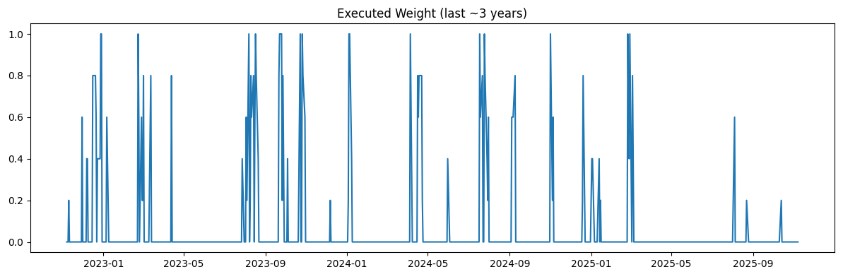
plt.figure(figsize=(12, 4))
plt.plot(df.loc[mask, "date"], w_exec.loc[mask])
plt.title("Executed Weight (last ~3 years)")
plt.tight_layout()
plt.show()
return res
# =============== Example Run ===============
if __name__ == "__main__":
code = 'nq'
path = fr"..\..\data\{code}.csv" # 예: r"C:/data/nq.csv"
price_df = pd.read_csv(path, parse_dates=["date"])
params = Params(
rpsi_window=10,
threshold=0.2,
sma_period=15,
vol_window=30,
z_limit=2.0,
lag_days=1,
csv_path=f"{code}_rpsi_volz2_result.csv",
show_plots=True,
weight_step=0.2,
fixed_ratio=0.0, # 고정비율투자
)
result = run_strategy(price_df, params)
print(result)
{'RPSI_Window': 10, 'Threshold': 0.2, 'Vol_Window': 30, 'Z_Limit': 2.0, 'CAGR': np.float64(0.045557033360181874), 'Sharpe': np.float64(0.763317044181156), 'MaxDD': -0.0750156760623577, 'Exposure(%)': 7.549407114624507, 'WinRate(%)': 7.060725835429393, 'Trades': 306, 'AvgHoldingDays': 2.2091503267973858, 'Final Equity': 1.0062319352490965, 'rpsi_window': 10, 'threshold': 0.2, 'sma_period': 15, 'vol_window': 30, 'z_limit': 2.0, 'lag_days': 1, 'csv_path': 'nq_rpsi_volz2_result.csv', 'show_plots': True, 'weight_step': 0.2, 'fixed_ratio': 0.0}
'시스템트레이딩' 카테고리의 다른 글
| Volatility Compression Filter (0) | 2025.11.16 |
|---|---|
| Target-Volatility Strategy - BTCKRW (0) | 2025.11.14 |
| 전략의 유효성 (0) | 2025.11.08 |
| Calm Rebound Allocator (CRA) (0) | 2025.11.07 |
| 자산배분전략의 환위험 헷지 (1) | 2025.11.06 |
